Guide Power Query
My table has a column for every month and nothing works
Twelve columns, one per month. It reads well on paper and it fights you in every other way: you cannot filter by month, you cannot pivot it, and each new month means editing every formula.
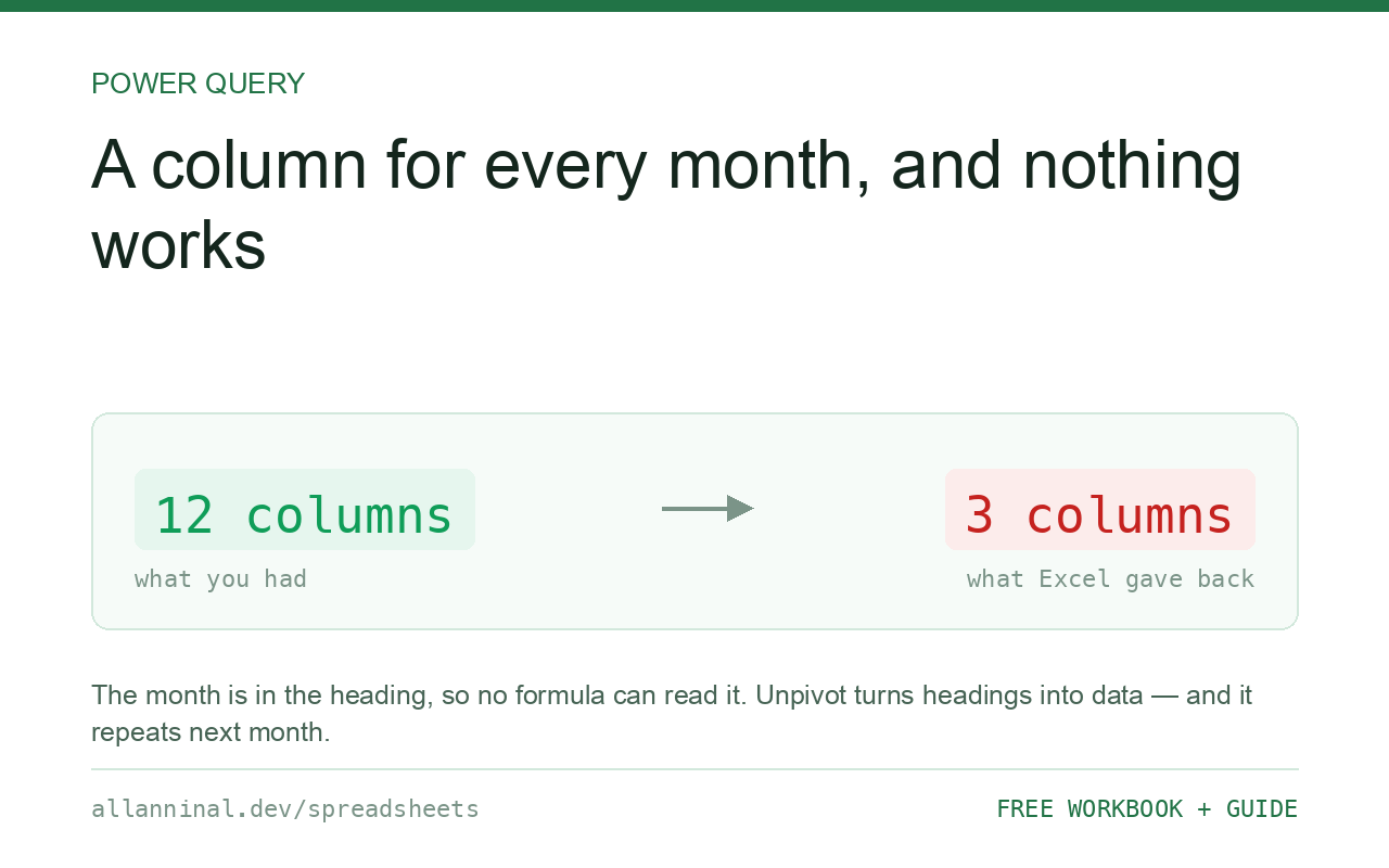
Select the columns you want to keep, right-click one of them and choose Unpivot Other Columns. Your twelve month columns collapse into two: one holding the month name and one holding the value. Get there with Data → From Table/Range to open Power Query first. Because Power Query saves the step, next month's file is fixed by pressing Refresh rather than doing it again.
Why a column per month makes everything harder
A wide table looks like a report. The trouble is that Excel's own tools — filters,
pivot tables, SUMIFS — all expect the opposite shape, where every row is one
observation and every column is one kind of thing.
With a column per month, the month is not in the data. It is in the column headings, and a formula cannot read a heading as easily as it reads a cell. So you end up writing twelve formulas instead of one, and adding a thirteenth by hand in January.
Unpivoting turns the headings into values. Three columns — who, which month, how much — and every tool in Excel starts working again.
| What you see | What actually happened | What fixes it |
|---|---|---|
| You cannot filter by month | The month is a heading, not a value | Unpivot so the month becomes data |
| A pivot table cannot use the months | Same reason — there is no month field | Unpivot first, then pivot |
| Twelve nearly identical formulas | One per column, because the column is the month | One SUMIFS after unpivoting |
| A new month means editing everything | The shape has to grow sideways | After unpivoting it grows downwards, which nothing breaks |
| Charts need re-pointing every month | The source range changed shape | A tall table keeps the same columns forever |
How to unpivot a table in Excel
Open the table in Power Query
Click any cell in the data, then Data → From Table/Range. If your range is not already a table Excel offers to make it one — say yes, and check My table has headers. The Power Query editor opens in its own window. Nothing has changed in your workbook yet.
Select the columns you want to KEEP
Click the heading of each column that identifies the row: product name, region, customer. Hold Ctrl to pick several. These are the columns that will stay as they are.
Do not select the month columns. That is the part people get backwards on the first try.
Right-click and choose Unpivot Other Columns
Right-click one of the highlighted headings and choose Unpivot Other Columns. Everything you did not select folds into two new columns called Attribute and Value.
Unpivot Other Columns rather than plain Unpivot Columns is the important choice: it means “fold up everything except these”, so a month column added next year is folded too, automatically.
Rename the two new columns
Double-click Attribute and type Month. Double-click
Value and type Amount. Then Close & Load to send the tidy table
back to a new sheet in your workbook.
Next month, just press Refresh
This is the part that matters. Power Query recorded what you did as a list of steps. Put next month's file in place and press Data → Refresh All, and the same steps run again in a second.
You did the work once. Everything after that is a button.
Everything on this page, as a workbook you can use on your own data
The Excel Data Cleanup Kit — a seven-tab workbook that finds all nine of these faults in a pasted column and hands back a cleaned version, a five-page PDF guide, and a short read-me. Free, no email required.
- Excel-Data-Cleanup-Workbook-Free.xlsx — paste a column, read the diagnosis, take the cleaned output
- Excel-Data-Survival-Guide.pdf — the eight failures, the import routine that prevents them, every formula explained
Plain .xlsx: no macros, no add-ins. Opens in Excel, Google Sheets,
Apple Numbers and LibreOffice Calc.
What "tidy" means, and why every tool wants it
There is a shape that spreadsheets and databases both prefer, and it has three rules:
- Every column is one kind of thing.
- Every row is one observation.
- Nothing important is stored in a heading.
A table with a column per month breaks the third rule, which is why it breaks the tools. Unpivoting is simply putting it back.
Going the other way
If you need the wide shape back — for a printed report, say — that is what a pivot table is for. Keep the tidy table as your data and let the pivot produce the layout. Never store the report shape and try to calculate from it.
Google Sheets does not have Power Query
There is no direct equivalent. The nearest is a formula that rebuilds the tall shape, or the
QUERY function. For a one-off, Sheets users often paste into Excel, unpivot, and paste
back — which is a fair use of ten minutes.
Two things that trip people up
- Blank cells become rows too. If a product had no sales in March you get a row with a blank amount. Filter them out inside Power Query with the arrow on the Amount heading.
- Months come back as text.
Jansorts beforeFebalphabetically, which is luck rather than order. If you need real dates, add a column that converts them while you are still in Power Query.
Questions people ask
What does unpivot mean?
It turns columns into rows. A table with twelve month columns becomes a table with a month column and a value column, so the month is data you can filter and pivot rather than a heading.
What is the difference between Unpivot Columns and Unpivot Other Columns?
Unpivot Columns folds up the ones you selected. Unpivot Other Columns folds up everything else. The second is safer, because a new column added later is included automatically.
Do I have to redo this every month?
No. Power Query saves your steps. Put the new file in place and press Data > Refresh All, and the same steps run again.
Does this change my original data?
No. Power Query reads your source and writes the result to a new sheet. The original is untouched.
Is Power Query available in my version of Excel?
It is built into Excel 2016 and later on Windows, and into Excel for Mac from 2019 onwards with some limits. In Excel 2010 and 2013 it was a free add-in from Microsoft.
Is there an equivalent in Google Sheets?
Not directly. Sheets has no Power Query. The nearest tools are the QUERY function or a formula that rebuilds the tall shape.
Related guides
Take the workbook with you
The Excel Data Cleanup Kit — a seven-tab workbook that finds all nine of these faults in a pasted column and hands back a cleaned version, a five-page PDF guide, and a short read-me. Free, no email required.
- Excel-Data-Cleanup-Workbook-Free.xlsx — paste a column, read the diagnosis, take the cleaned output
- Excel-Data-Survival-Guide.pdf — the eight failures, the import routine that prevents them, every formula explained
Plain .xlsx: no macros, no add-ins. Opens in Excel, Google Sheets,
Apple Numbers and LibreOffice Calc.