Guide Formulas
I need a total for each category
Sales by region, hours by project, spend by supplier. Excel has two good answers and they suit genuinely different jobs — one is a formula that lives in your layout, the other is a tool for looking around.
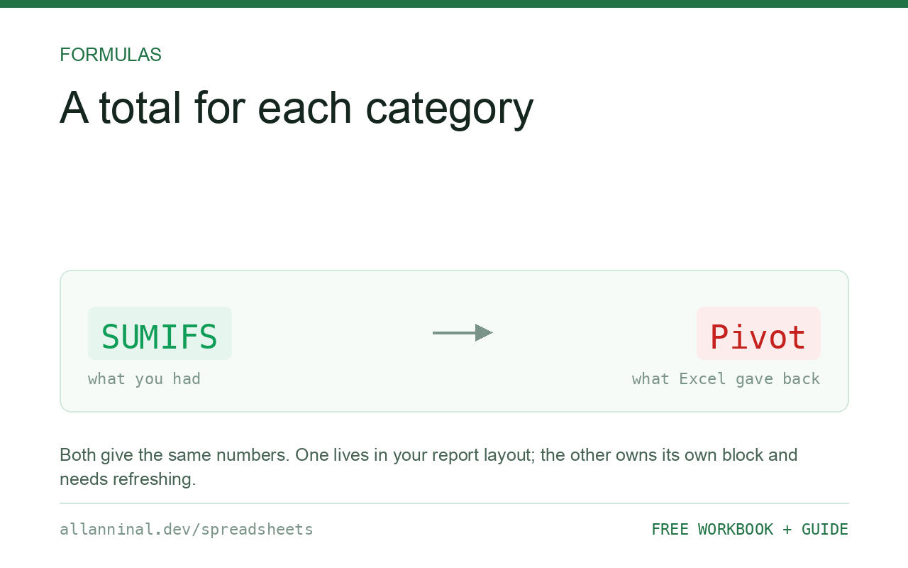
Use SUMIFS when the answer belongs in a report you control
and must update automatically; use a pivot table when you are exploring and do not yet know which
breakdown you want. =SUMIFS(Amount,Region,"North") totals one category and
recalculates on its own. A pivot table produces every category at once but must be refreshed by
hand.
The real difference is who controls the layout
Both give the same numbers. They differ in what happens next.
A pivot table owns its own block of the sheet. You cannot put a column of your own in the middle of it, and its shape changes as the data changes. That is exactly what you want when exploring — drag a field, see a different cut — and exactly what you do not want inside a monthly report with a fixed layout.
SUMIFS lives wherever you put it. The row labels are yours, the
formatting is yours, and the figure updates the moment the data changes. That is what a report needs,
and it is why finance models are full of SUMIFS and short of pivot tables.
The pivot table's real weakness is the refresh. It shows a cached result until someone right-clicks
and chooses Refresh, so a printed report can be silently out of date. SUMIFS cannot be
stale (unless calculation is set to Manual).
| What you see | What actually happened | What fixes it |
|---|---|---|
SUMIFS returns 0 | The criterion does not match exactly, or the values are text | Check for spaces and check the type |
| Pivot total does not match the data | The pivot is showing a cached result | Right-click → Refresh |
| New rows missing from the pivot | They fell outside the source range | Base the pivot on a table (Ctrl+T) |
#VALUE! from SUMIFS | The sum range and criteria ranges are different sizes | Make every range the same height |
| Categories split that should be together | Trailing spaces or inconsistent capitalisation | Clean the category column |
How to total by category in Excel
Build the category list first
You need somewhere for the totals to sit. On 365,
=SORT(UNIQUE(Data!C2:C5000)) gives you the row labels and keeps them current; on older
Excel use Advanced Filter.
Total each one with SUMIFS
Point the criterion at your label cell rather than typing the category into the formula:
=SUMIFS(Data!$D$2:$D$5000,Data!$C$2:$C$5000,$A2)Sum range first, then pairs of range and criterion. $A2 is a mixed
reference so it follows the row but not the column — that is what lets one formula fill the
whole report.
Add more conditions as more pairs
Every extra condition is another range-and-criterion pair:
=SUMIFS(Data!$D$2:$D$5000,Data!$C$2:$C$5000,$A2,
        Data!$B$2:$B$5000,">="&$B$1,Data!$B$2:$B$5000,"<="&$B$2)
Note ">="&$B$1 — the operator is a string, joined to the
cell reference with &. Typing ">=$B$1" instead compares against the
literal text and silently returns zero.
For exploring, use a pivot table on a real table
Press Ctrl+T on your data first, then Insert →
PivotTable. A table source expands as rows are added, so new data appears on refresh. A fixed
range like A1:D5000 silently ignores row 5001 forever — the most common reason a
pivot total is quietly wrong.
Everything on this page, as a workbook you can use on your own data
The Excel Data Cleanup Kit — a seven-tab workbook that finds all nine of these faults in a pasted column and hands back a cleaned version, a five-page PDF guide, and a short read-me. Free, no email required.
- Excel-Data-Cleanup-Workbook-Free.xlsx — paste a column, read the diagnosis, take the cleaned output
- Excel-Data-Survival-Guide.pdf — the eight failures, the import routine that prevents them, every formula explained
Plain .xlsx: no macros, no add-ins. Opens in Excel, Google Sheets,
Apple Numbers and LibreOffice Calc.
Why SUMIFS returns zero
Nearly always one of three things:
- The category has a trailing space in the data but not in your label, so nothing matches.
- The sum column is text, not numbers —
SUMIFSskips text exactly asSUMdoes. - The operator is inside the quotes:
">=$B$1"instead of">="&$B$1. The first compares against a literal string and matches nothing.
SUMIF and SUMIFS put their arguments in different orders
This catches everyone. SUMIF(range, criterion, sum_range) puts the sum range
last. SUMIFS(sum_range, range1, criterion1, ...) puts it first. Use
SUMIFS for everything, even with one condition, and the inconsistency stops mattering.
Counting and averaging work the same way
COUNTIFS and AVERAGEIFS take the same argument shape. AVERAGEIFS
returns #DIV/0! when nothing matches, so wrap it in IFERROR if empty
categories are expected.
Google Sheets has a third option
Sheets has SUMIFS and pivot tables too, plus QUERY, which does
SQL-style grouping in a single formula:
=QUERY(A:D,"select C, sum(D) group by C"). Excel has no equivalent.
Questions people ask
Should I use SUMIFS or a pivot table?
SUMIFS when the number belongs in a report layout you control and must update automatically. A pivot table when you are exploring the data and do not yet know which breakdown you need.
Why does my SUMIFS return zero?
Usually a trailing space on the category, a sum column stored as text, or an operator written inside the quotes as ">=$B$1" instead of ">="&$B$1.
Why is my pivot table total wrong?
It is showing a cached result and needs refreshing, or new rows fell outside a fixed source range. Base the pivot on a table created with Ctrl+T so it grows automatically.
What is the difference between SUMIF and SUMIFS?
The argument order. SUMIF takes the sum range last; SUMIFS takes it first. Use SUMIFS for everything, even single conditions, and the inconsistency stops being a problem.
How many conditions can SUMIFS handle?
Up to 127 criteria pairs. Every range must be the same height as the sum range or you get a #VALUE! error.
Is there a SQL-style GROUP BY in Excel?
Not natively. Google Sheets has QUERY, which does it in one formula. In Excel the equivalent is SUMIFS, a pivot table, or Power Query's Group By step.
Related guides
Take the workbook with you
The Excel Data Cleanup Kit — a seven-tab workbook that finds all nine of these faults in a pasted column and hands back a cleaned version, a five-page PDF guide, and a short read-me. Free, no email required.
- Excel-Data-Cleanup-Workbook-Free.xlsx — paste a column, read the diagnosis, take the cleaned output
- Excel-Data-Survival-Guide.pdf — the eight failures, the import routine that prevents them, every formula explained
Plain .xlsx: no macros, no add-ins. Opens in Excel, Google Sheets,
Apple Numbers and LibreOffice Calc.