Guide Dynamic arrays
I want every row that matches, not just the first
A lookup gives you one answer. FILTER gives you all of them, as a list that updates itself — and then shows a column of zeros where your data had blanks, which is where most people stop.
=FILTER(range, condition, "none") returns every row where
the condition is true. Combine conditions with * for AND and + for
OR — not the words. Always give the third argument, or an empty result shows
#CALC!. Blank cells in the source come back as 0, because an empty cell is
zero to Excel; wrap the result in IF(result="","",result) if that matters.
Two surprises, both worth knowing before you start
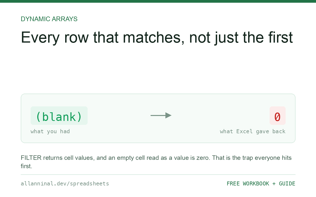
Blanks become zeros. FILTER returns cell values, and an
empty cell read as a value is 0. So a filtered list of customers shows 0
wherever the phone number was missing. Nothing is wrong; it is Excel's ordinary treatment of empty
cells, surfacing where you can finally see it.
AND and OR do not work here. Those functions collapse a
whole range into a single TRUE or FALSE, so FILTER receives one answer instead of one
per row and returns everything or nothing. You need * for AND and + for OR,
which multiply and add the TRUE/FALSE values row by row.
Neither is documented anywhere you will look at the moment you need it.
| What you see | What actually happened | What fixes it |
|---|---|---|
| Zeros where the source was blank | An empty cell read as a value is 0 | Wrap in IF(x="","",x) |
#CALC! | Nothing matched and there is no third argument | Add ,"none found" |
| Every row returned | AND collapsed the test to one TRUE | Use * between conditions |
#VALUE! | The condition is a different height from the range | Make both the same number of rows |
#NAME? | Your version does not have FILTER | Use an advanced filter or a pivot table |
How to use FILTER
Start with one condition
The range you want back, then the test:
=FILTER(A2:D500,B2:B500="Acme Ltd","none found")The third argument is what to show when nothing matches. Always include it. Without
it an empty result is #CALC!, which looks like a broken formula rather than a clean
answer of “none”.
Combine conditions with * and +
Multiplication is AND, addition is OR:
=FILTER(A2:D500,(B2:B500="Acme")*(C2:C500>1000),"none")
=FILTER(A2:D500,(B2:B500="Acme")+(B2:B500="Northwind"),"none")
TRUE behaves as 1 and FALSE as 0, so multiplying gives 1 only when both hold, and adding gives at least 1 when either does. Bracket each condition — without brackets the operator precedence quietly changes what you asked for.
Turn the zeros back into blanks
If the zeros are misleading — a phone number of 0 is worse than no phone number — swap them back:
=LET(r,FILTER(A2:D500,B2:B500="Acme","none"),IF(r="","",r))LET names the result so FILTER runs once rather than twice.
Without LET you would write the whole formula twice and it would do the work twice.
Sort the result while you are at it
FILTER returns rows in their original order. Wrap it to change
that:
=SORT(FILTER(A2:D500,B2:B500="Acme","none"),3,-1)Sort by the third column, descending. The two functions compose in either order but this way round reads more naturally: filter first, then sort what is left.
Everything on this page, as a workbook you can use on your own data
The Excel Data Cleanup Kit — a seven-tab workbook that finds all nine of these faults in a pasted column and hands back a cleaned version, a five-page PDF guide, and a short read-me. Free, no email required.
- Excel-Data-Cleanup-Workbook-Free.xlsx — paste a column, read the diagnosis, take the cleaned output
- Excel-Data-Survival-Guide.pdf — the eight failures, the import routine that prevents them, every formula explained
Plain .xlsx: no macros, no add-ins. Opens in Excel, Google Sheets,
Apple Numbers and LibreOffice Calc.
Filtering by a cell instead of typed text
Point the condition at a cell and the list becomes interactive — type a different customer
in G1 and the results change:
=FILTER(A2:D500,B2:B500=G1,"no orders for that customer")Add a dropdown on G1 with Data → Data Validation and you have built
a small search tool with one formula and no code.
Filtering on a partial match
FILTER tests for equality, so it will not do “contains” on its own. Pair
it with SEARCH:
=FILTER(A2:D500,ISNUMBER(SEARCH("ltd",B2:B500)),"none")SEARCH returns a position or an error, and ISNUMBER turns that into
the TRUE/FALSE per row that FILTER needs. SEARCH ignores capitals;
FIND does not.
What to do without FILTER
On Excel 2019 or earlier, the honest answers are Data → Advanced Filter, which copies
matching rows somewhere else, or a pivot table. The array formulas that simulate
FILTER are long, slow and hard for the next person to maintain.
Google Sheets
Sheets has FILTER and has had it far longer. The differences are worth knowing: it
takes no third argument, so an empty result is #N/A and you wrap it in
IFERROR; and it accepts multiple conditions as extra arguments rather than needing
*.
Questions people ask
Why does FILTER return 0 for blank cells?
An empty cell read as a value is zero to Excel. Wrap the result in IF(result="","",result) to keep blanks looking blank.
What does #CALC! mean?
Nothing matched and you did not supply the third argument. Add something like "none found" and an empty result becomes readable instead of an error.
Why does AND not work inside FILTER?
AND collapses a whole range into a single TRUE or FALSE, so FILTER gets one answer rather than one per row. Multiply conditions with * for AND and add them with + for OR.
How do I filter on 'contains' rather than an exact match?
Use ISNUMBER(SEARCH("word",range)) as the condition. SEARCH ignores capitals; FIND does not.
What can I use instead on older Excel?
Data > Advanced Filter, which copies matching rows elsewhere, or a pivot table. The array formulas that imitate FILTER are slow and hard to maintain.
Is Google Sheets FILTER the same?
Close but not identical. Sheets takes no third argument, so wrap it in IFERROR, and it accepts several conditions as extra arguments rather than needing *.
Related guides
Take the workbook with you
The Excel Data Cleanup Kit — a seven-tab workbook that finds all nine of these faults in a pasted column and hands back a cleaned version, a five-page PDF guide, and a short read-me. Free, no email required.
- Excel-Data-Cleanup-Workbook-Free.xlsx — paste a column, read the diagnosis, take the cleaned output
- Excel-Data-Survival-Guide.pdf — the eight failures, the import routine that prevents them, every formula explained
Plain .xlsx: no macros, no add-ins. Opens in Excel, Google Sheets,
Apple Numbers and LibreOffice Calc.