Guide Formulas
Which of these names are missing from the other list?
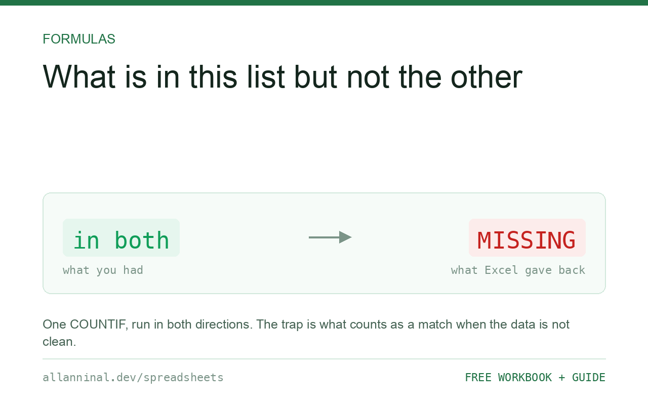
Two lists that should agree and do not: a stock count against the system, a bank statement against the ledger, this month's members against last month's. The comparison itself is one formula — the trap is what counts as a match.
=COUNTIF(ListB,A2)=0 is TRUE when the value in
A2 does not appear in list B. It works in every version of Excel, in Google
Sheets and in LibreOffice. On Microsoft 365,
=FILTER(A2:A500,COUNTIF(B2:B500,A2:A500)=0) returns the missing items as a list in one
step. Run it in both directions — A-not-in-B and B-not-in-A are different questions with
different answers.
Both directions, and the reason matches fail
Two mistakes account for nearly every wrong answer here.
Only checking one direction. “What is in A but not B” does not tell you what is in B but not A. A stock count that finds no missing items may still contain items that should not exist at all. Always run both.
Comparing dirty values. COUNTIF matches exactly as stored, so a
trailing space, a non-breaking space, or one side stored as text and the other as a number all
produce a confident MISSING for a row that is sitting right there. In a reconciliation, that is worse
than no answer — it sends someone hunting for a discrepancy that does not exist.
| What you see | What actually happened | What fixes it |
|---|---|---|
| Everything reports as missing | One list is text, the other numbers | Make both the same type |
| A handful wrongly missing | Invisible characters on one side | Clean both columns first |
#NAME? from FILTER | Not available in your Excel version | Use the COUNTIF method |
| Counts do not agree with the list | Duplicates counted more than once | Deduplicate before comparing |
| Matches ignore capitalisation | COUNTIF is not case-sensitive | Use SUMPRODUCT with EXACT |
How to compare two lists in Excel
Flag what is missing, in both directions
Beside list A:
=IF(COUNTIF($B$2:$B$500,A2)=0,"MISSING FROM B","ok")And the mirror image beside list B, pointing at column A. Two columns, two questions, two different answers.
On Microsoft 365, get the list directly
No helper column, and it stays live:
=FILTER(A2:A500,COUNTIF(B2:B500,A2:A500)=0,"none missing")The third argument is what to show when nothing is missing — without it you get
#CALC!, which looks like a failure rather than a clean result.
Clean both sides before you trust the answer
Add a cleaned helper column beside each list and compare those:
=IF(COUNTIF($D$2:$D$500,TRIM(A2))=0,"MISSING","ok")Where column D holds the cleaned version of list B. If the two lists came from different systems, assume they need cleaning — they almost always do.
Check the types match
An order number stored as text in one export and as a number in the other will never
match, however clean both are. Test with =ISTEXT(A2) on each side. Convert one, or
compare TEXT(A2,"@") against TEXT(B2,"@") so both are strings.
Everything on this page, as a workbook you can use on your own data
The Excel Data Cleanup Kit — a seven-tab workbook that finds all nine of these faults in a pasted column and hands back a cleaned version, a five-page PDF guide, and a short read-me. Free, no email required.
- Excel-Data-Cleanup-Workbook-Free.xlsx — paste a column, read the diagnosis, take the cleaned output
- Excel-Data-Survival-Guide.pdf — the eight failures, the import routine that prevents them, every formula explained
Plain .xlsx: no macros, no add-ins. Opens in Excel, Google Sheets,
Apple Numbers and LibreOffice Calc.
Highlighting the differences visually
For a quick visual answer, conditional formatting takes the same formula. Select list A, Home → Conditional Formatting → New Rule → Use a formula, and enter:
=COUNTIF($B$2:$B$500,A2)=0Pick a fill colour and every unmatched value in A is highlighted. Note the mixed reference
— $B$2:$B$500 pinned, A2 relative — which is what lets the rule
walk down the column.
Case-sensitive comparison
COUNTIF ignores capitalisation. Where ABC123 and abc123 are
genuinely different codes, use:
=SUMPRODUCT(--EXACT($B$2:$B$500,A2))=0EXACT compares case as well as characters, and SUMPRODUCT counts how
many exact matches exist.
Matching on more than one column
When identity depends on two fields — a date and an amount, a first name
and a surname — use COUNTIFS with a criterion per column rather than
concatenating the fields into a key. Concatenation creates false matches whenever one value ends
where the next begins.
When the lists are large
COUNTIF across two columns of 100,000 rows is slow, because it is comparing every
value against every value. Sort both lists first, or use MATCH, which stops at the first
hit and is noticeably faster on large ranges.
Questions people ask
How do I find values in one column that are not in another?
Use =COUNTIF(OtherList,A2)=0. TRUE means the value does not appear in the other list. On Microsoft 365, FILTER with the same COUNTIF test returns the missing items as a list.
Do I need to compare in both directions?
Yes. What is in A but not B is a different question from what is in B but not A, and a reconciliation needs both answers.
Why does everything report as missing?
Usually a type mismatch — one list holds numbers and the other holds text versions of the same values. They never match, however clean both are.
Why do a few rows wrongly report as missing?
Invisible characters, typically a trailing or non-breaking space on one side. COUNTIF compares values exactly as stored, so clean both columns first.
Is COUNTIF case-sensitive?
No. For a case-sensitive comparison use =SUMPRODUCT(--EXACT(Range,A2))=0, which compares capitalisation as well as characters.
How do I match on two columns at once?
Use COUNTIFS with one criterion per column. Concatenating the columns into a single key creates false matches where one value ends and the next begins.
Related guides
Take the workbook with you
The Excel Data Cleanup Kit — a seven-tab workbook that finds all nine of these faults in a pasted column and hands back a cleaned version, a five-page PDF guide, and a short read-me. Free, no email required.
- Excel-Data-Cleanup-Workbook-Free.xlsx — paste a column, read the diagnosis, take the cleaned output
- Excel-Data-Survival-Guide.pdf — the eight failures, the import routine that prevents them, every formula explained
Plain .xlsx: no macros, no add-ins. Opens in Excel, Google Sheets,
Apple Numbers and LibreOffice Calc.