Guide Formulas
I need to pull data from one sheet into another
You have orders in one sheet and customers in another, joined by an ID. In SQL this is a join. In Excel it is a lookup, and which function you pick decides how badly it breaks when someone inserts a column.
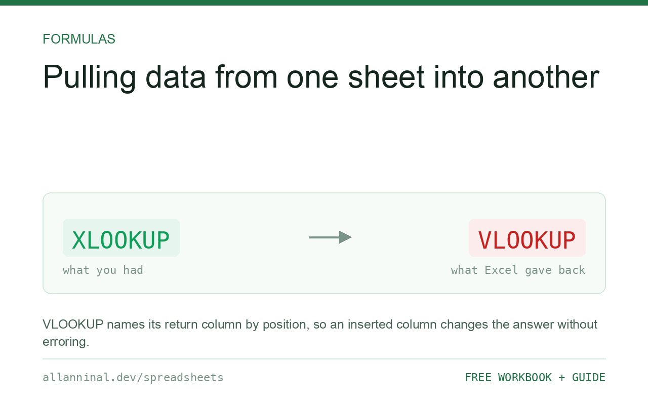
Use XLOOKUP if you have Microsoft 365 or Excel 2021, and
INDEX/MATCH otherwise.
=XLOOKUP(A2,Customers!$A:$A,Customers!$C:$C,"not found") pulls a value across, handles
the not-found case in the formula, and does not care where the columns sit. VLOOKUP
works but refers to the return column by position, so inserting a column silently changes
what it returns.
Why VLOOKUP breaks and the others do not
VLOOKUP's third argument is a column number. Written as
VLOOKUP(A2,Customers!A:F,3,FALSE), it means “the third column of that range”.
Insert a new column anywhere inside that range — something a colleague may do for entirely good reasons — and the third column is now a different field. The formula does not error. It returns the wrong data, confidently, and there is nothing on screen to indicate it.
XLOOKUP and INDEX/MATCH both refer to the return column by
reference, so an inserted column shifts the reference with it and the formula keeps
returning the same field. This is the whole reason to move off VLOOKUP.
VLOOKUP also cannot look to its left: the key must be in the first column of the
range. XLOOKUP and INDEX/MATCH have no such restriction.
| What you see | What actually happened | What fixes it |
|---|---|---|
| #N/A on rows you can see exist | Invisible characters, or a type mismatch | Clean both key columns and check types |
| Wrong data after someone edited the other sheet | VLOOKUP's column index now points elsewhere | Switch to XLOOKUP or INDEX/MATCH |
| #REF! in the formula | The column index is beyond the range | Check the range covers the return column |
| Returns the first match only | Lookups return one value by design | Use FILTER, or aggregate with SUMIFS |
| Workbook became very slow | Thousands of lookups over whole-column ranges | Limit ranges, or use Power Query to merge |
How to look up data from another sheet
Microsoft 365: use XLOOKUP
Four arguments, in a readable order:
=XLOOKUP(A2,Customers!$A:$A,Customers!$C:$C,"not found")Lookup value, where to search, what to return, and the not-found result. Exact match is
the default — unlike VLOOKUP, where forgetting FALSE gives you an
approximate match and quietly wrong answers.
Older Excel: use INDEX and MATCH
Read it inside out: MATCH finds the row, INDEX fetches
from it.
=IFERROR(INDEX(Customers!$C:$C,MATCH(A2,Customers!$A:$A,0)),"not found")The 0 in MATCH means exact match and is not optional —
without it you get an approximate match against unsorted data, which returns nonsense. Works in every
version of Excel, in Sheets and in LibreOffice.
Always handle the not-found case
A column of #N/A makes every downstream SUM fail too.
XLOOKUP takes the fallback as its fourth argument; for
INDEX/MATCH use IFERROR.
Use a specific label such as "no customer record" rather than an empty string. A blank
tells you nothing about whether the lookup failed or the source was genuinely empty.
Check the key columns are the same type
This is the most common cause of a lookup that fails on every row. Test both sides:
=ISTEXT(A2) =ISTEXT(Customers!A2)Different answers mean no row will ever match. Convert one side, or wrap both in
TEXT(...,"@") so the comparison is string to string.
Everything on this page, as a workbook you can use on your own data
The Excel Data Cleanup Kit — a seven-tab workbook that finds all nine of these faults in a pasted column and hands back a cleaned version, a five-page PDF guide, and a short read-me. Free, no email required.
- Excel-Data-Cleanup-Workbook-Free.xlsx — paste a column, read the diagnosis, take the cleaned output
- Excel-Data-Survival-Guide.pdf — the eight failures, the import routine that prevents them, every formula explained
Plain .xlsx: no macros, no add-ins. Opens in Excel, Google Sheets,
Apple Numbers and LibreOffice Calc.
When you need more than one match
Lookups return a single value. To bring back every matching row — all orders for a
customer, say — use FILTER on Microsoft 365:
=FILTER(Orders!$A:$D,Orders!$B:$B=A2,"no orders")On older Excel there is no clean formula for this. Use a pivot table, or aggregate instead of
listing: SUMIFS for a total, COUNTIFS for a count.
Power Query is the real join
For a genuine table-to-table join, Power Query is the right tool and almost nobody reaches for it. Data → Get Data → Combine Queries → Merge gives you inner, left, right, full outer and anti joins by name — the same vocabulary as SQL.
It is also dramatically faster. Fifty thousand XLOOKUP formulas recalculate on every
change; a merged query is computed once on refresh. If your workbook has slowed to a crawl from
lookups, this is the fix.
Clean the keys first
Everything here assumes the two key columns actually match. In practice they usually do not — different systems, different exports, different amounts of whitespace. Clean both sides before you conclude a record is missing.
Questions people ask
Should I use VLOOKUP or XLOOKUP?
XLOOKUP if you have it. It refers to the return column by reference rather than by position, so an inserted column cannot silently change what the formula returns, and it can look to the left.
What is the equivalent of a SQL join in Excel?
For a single column, a lookup. For a genuine table-to-table join, Power Query's Merge, which offers inner, left, right, full outer and anti joins by name.
Why does my VLOOKUP return the wrong column?
Its third argument is a column number, not a reference. Inserting a column inside the range changes which field that number points at, and the formula returns wrong data without erroring.
How do I return every matching row rather than the first?
Use FILTER on Microsoft 365. On older Excel there is no clean formula — use a pivot table, or aggregate with SUMIFS or COUNTIFS instead of listing.
Why does every row return #N/A?
Most often the key is text on one side and a number on the other, so nothing can match. Check with ISTEXT on both sides. Invisible characters are the other common cause.
My workbook is very slow with lookups. What should I do?
Avoid whole-column ranges, and consider replacing the lookups with a Power Query merge, which computes once on refresh rather than on every recalculation.
Related guides
Take the workbook with you
The Excel Data Cleanup Kit — a seven-tab workbook that finds all nine of these faults in a pasted column and hands back a cleaned version, a five-page PDF guide, and a short read-me. Free, no email required.
- Excel-Data-Cleanup-Workbook-Free.xlsx — paste a column, read the diagnosis, take the cleaned output
- Excel-Data-Survival-Guide.pdf — the eight failures, the import routine that prevents them, every formula explained
Plain .xlsx: no macros, no add-ins. Opens in Excel, Google Sheets,
Apple Numbers and LibreOffice Calc.