Guide Conditional formatting
Colour this cell based on what that cell says
Highlight the row when the status column says Overdue. Colour the amount when it is over budget. The built-in rules cannot do it — you need a formula rule, and one detail decides whether it works.
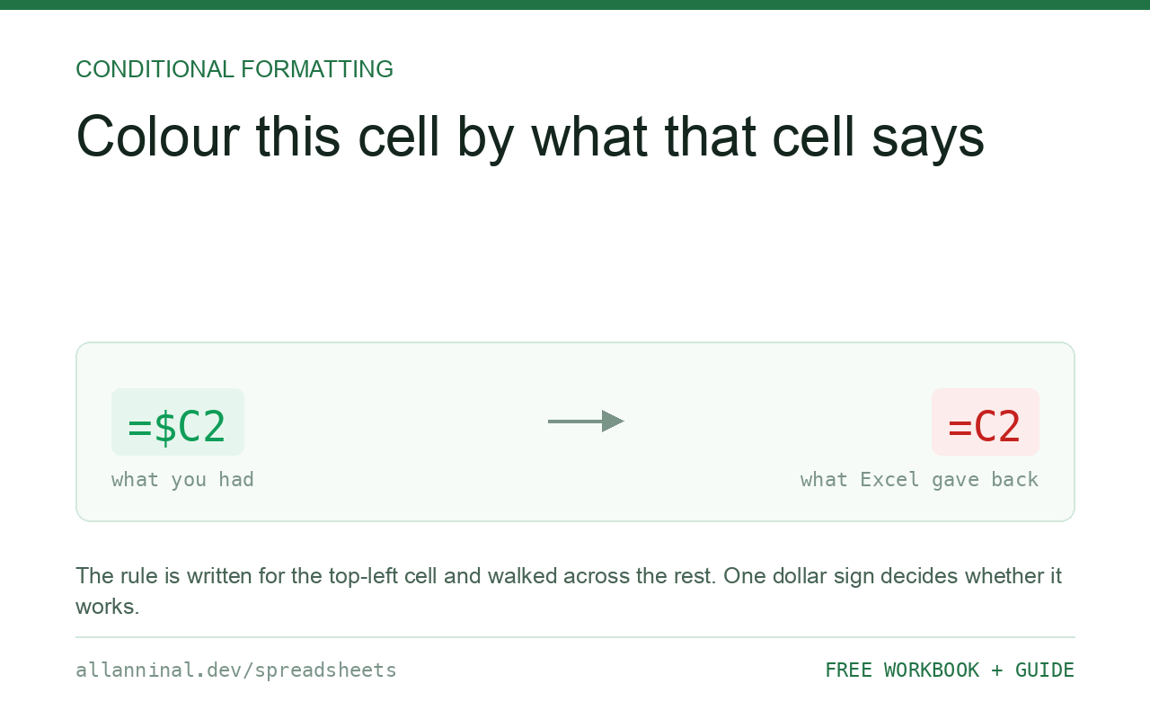
Use Home → Conditional Formatting → New Rule → Use a
formula, and write the formula as if for the top-left cell of your selection only.
Excel applies it to every other cell by shifting the references, exactly as it would if you dragged a
formula. So lock the column with a dollar sign — =$C2="Overdue" — and the
whole row follows column C.
The rule is written once and walked across everything
This is the whole idea, and nothing in the dialog explains it.
You select a range and write one formula. Excel applies that formula to the top-left cell of the selection, then moves it to every other cell in exactly the way dragging a formula would: relative references shift, and anything with a dollar sign in front of it does not.
So if you select A2:F100 and write =C2="Overdue", cell B2
tests D2, and C2 tests E2. Every cell tests a different column,
and the colours look random.
Writing =$C2="Overdue" pins the column and lets the row move. Now every cell in row 2
tests C2, every cell in row 3 tests C3, and the whole row lights up
together.
| What you see | What actually happened | What fixes it |
|---|---|---|
| Only the first column colours | The reference is fully absolute — $C$2 | Free the row: $C2 |
| Colours look scattered at random | Nothing is pinned, so every cell tests a different column | Pin the column: $C2 |
| Nothing highlights at all | The formula was written for the wrong row | Write it for the FIRST row of the selection |
| Correct at first, wrong after inserting rows | The Applies To range shifted | Fix it in Manage Rules |
| The rule split into dozens of rules | Copy and paste fragmented the range | Delete them all and reapply once |
How to format a row based on another cell
Select the whole range you want coloured, starting at the top left
To colour whole rows, select A2:F100, not column C. Start the selection
at A2, because that is the cell your formula will describe.
Do not include the header row unless you want it coloured too.
Add a formula rule
Home → Conditional Formatting → New Rule → Use a formula to determine which cells to format. It is the last option in the list and the only one that can look at a different cell.
Write the formula for the top-left cell, pinning the column
For a selection starting at A2, testing column C:
=$C2="Overdue"The $ before C stops the column moving as the rule walks
sideways. No $ before 2 lets the row move as it walks down. That is the
entire trick.
Check the Applies To range afterwards
Conditional Formatting → Manage Rules, and look at Applies to. It should be your whole range. Copying and pasting cells inside the range tends to shatter one rule into several with odd fragments — when that happens, delete them all and apply once, cleanly.
Everything on this page, as a workbook you can use on your own data
The Excel Data Cleanup Kit — a seven-tab workbook that finds all nine of these faults in a pasted column and hands back a cleaned version, a five-page PDF guide, and a short read-me. Free, no email required.
- Excel-Data-Cleanup-Workbook-Free.xlsx — paste a column, read the diagnosis, take the cleaned output
- Excel-Data-Survival-Guide.pdf — the eight failures, the import routine that prevents them, every formula explained
Plain .xlsx: no macros, no add-ins. Opens in Excel, Google Sheets,
Apple Numbers and LibreOffice Calc.
Useful rules to keep
- Overdue:
=AND($D2<TODAY(),$E2="")— due date passed and nothing in the completed column. - Over budget:
=$C2>$B2— actual above planned. - Blank required field:
=$B2="". - Top ten percent:
=$D2>=PERCENTILE($D$2:$D$100,0.9)— note the range is fully pinned, because it is the same range for every row. - Weekend:
=WEEKDAY($A2,2)>5.
Banding a table by group
To shade alternate groups rather than alternate rows, count the distinct values above and test whether that count is even. It is a rule that reads badly and looks excellent on a sorted report.
Rules run in order, and can stop
In Manage Rules, rules are applied top to bottom and later ones can overwrite earlier ones. The Stop If True checkbox halts processing for a cell when a rule matches — useful for “if it is cancelled, grey it out and ignore every other rule”.
Google Sheets
Same idea, called Custom formula is under Format → Conditional formatting. The dollar-sign behaviour is identical. Sheets applies the rule relative to the top-left of the range you gave it, exactly as Excel does.
Questions people ask
How do I highlight a whole row based on one cell?
Select the whole range, add a formula rule, and write it for the top-left cell with the column pinned — for example =$C2="Overdue". Pinning the column is what makes the whole row follow column C.
Why do only some cells change colour?
The references are wrong for how the rule walks. Fully absolute ($C$2) colours only where that one cell matches; nothing pinned makes every cell test a different column.
Which cell should the formula be written for?
The top-left cell of the range you selected. Excel applies it there and shifts the references for every other cell, exactly like dragging a formula.
Why did my rule stop working after I inserted rows?
The Applies To range shifted. Open Manage Rules and check it still covers the whole range.
Why has one rule turned into twenty?
Copying and pasting cells inside the range fragments the rule. Delete all the fragments and apply the rule once over the whole range.
Does this work the same in Google Sheets?
Yes. It is called Custom formula is, and the dollar-sign behaviour is identical.
Related guides
Take the workbook with you
The Excel Data Cleanup Kit — a seven-tab workbook that finds all nine of these faults in a pasted column and hands back a cleaned version, a five-page PDF guide, and a short read-me. Free, no email required.
- Excel-Data-Cleanup-Workbook-Free.xlsx — paste a column, read the diagnosis, take the cleaned output
- Excel-Data-Survival-Guide.pdf — the eight failures, the import routine that prevents them, every formula explained
Plain .xlsx: no macros, no add-ins. Opens in Excel, Google Sheets,
Apple Numbers and LibreOffice Calc.