Guide Conditional formatting
Show me which of these appear more than once
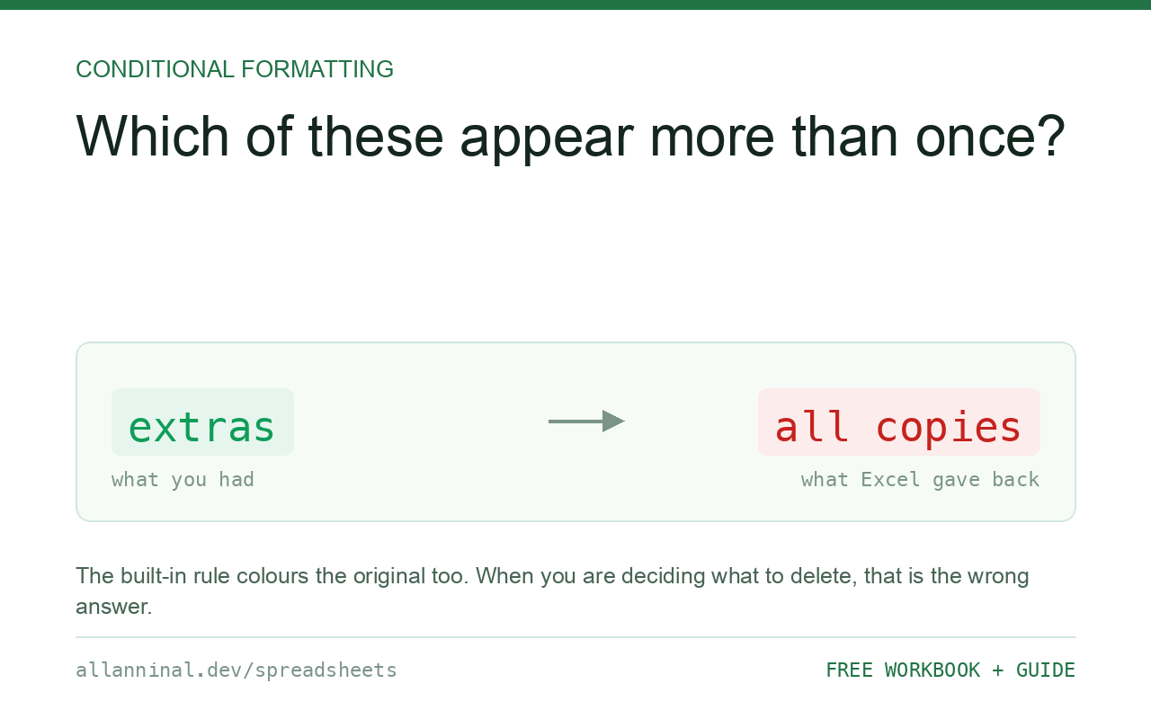
The built-in rule handles a single column and colours every copy, including the first. Most of the time what you actually want is subtler than that.
For one column, Home → Conditional Formatting → Highlight
Cells Rules → Duplicate Values is enough. For anything else, use a formula rule
with COUNTIF: =COUNTIF($A$2:$A$500,$A2)>1 flags every copy, and
=COUNTIF($A$2:$A2,$A2)>1 flags only the second and later — note the range that
grows as the rule walks down.
What the built-in rule cannot do
It is a good rule with three real limits, and each of them matters in practice.
- It colours every copy, including the first. When you are deciding what to delete, that is unhelpful — you want the extras marked, not the original.
- It works on one column at a time. A duplicate defined by name and date together is beyond it.
- It ignores capitals.
ACMEandacmeare duplicates to it. Sometimes right, sometimes very wrong.
All three are solved by a formula rule, and all three use COUNTIF in slightly
different ways.
| What you see | What actually happened | What fixes it |
|---|---|---|
| Every copy is highlighted | The built-in rule colours all of them | Use a growing range to flag the extras only |
| Duplicates not detected | Trailing or non-breaking spaces | Clean the column first |
| Numbers not matching text versions | Different types are never equal | Make both the same type |
| Long codes wrongly flagged | COUNTIF compares only the first 15 digits | Compare with &"" appended |
| Very slow on a large sheet | COUNTIF over a whole column, per cell | Bound the range to the rows in use |
How to highlight duplicates
One column, every copy: use the built-in rule
Select the column, then Home → Conditional Formatting → Highlight Cells Rules → Duplicate Values. Two clicks, and for a quick look it is the right tool.
Flag only the second and later copies
The range grows as the rule walks down, which is what makes this work:
=COUNTIF($A$2:$A2,$A2)>1$A$2 is pinned and $A2 is not, so on row 5 the range is
$A$2:$A5. The first occurrence sees a count of 1 and stays uncoloured; every later one
sees 2 or more. This is the rule to use before deleting anything.
Duplicates across two columns
When identity depends on two fields:
=COUNTIFS($A$2:$A$500,$A2,$B$2:$B$500,$B2)>1Select both columns before applying it. Use COUNTIFS rather than joining
the two values into one string — joining creates false matches where one value ends and the
next begins.
Case-sensitive duplicates
Where case carries meaning:
=SUMPRODUCT(--EXACT($A$2:$A$500,$A2))>1EXACT compares capitals as well as characters. Slower than
COUNTIF, so bound the range.
Everything on this page, as a workbook you can use on your own data
The Excel Data Cleanup Kit — a seven-tab workbook that finds all nine of these faults in a pasted column and hands back a cleaned version, a five-page PDF guide, and a short read-me. Free, no email required.
- Excel-Data-Cleanup-Workbook-Free.xlsx — paste a column, read the diagnosis, take the cleaned output
- Excel-Data-Survival-Guide.pdf — the eight failures, the import routine that prevents them, every formula explained
Plain .xlsx: no macros, no add-ins. Opens in Excel, Google Sheets,
Apple Numbers and LibreOffice Calc.
Highlighting the whole duplicate row
Select the full width of the data and pin the column being tested:
=COUNTIF($A$2:$A$500,$A2)>1Applied to A2:F500, this colours the entire row for each duplicate, because the
$ before A keeps every cell in the row looking at column A.
The 15-digit trap
COUNTIF compares numbers with about 15 digits of precision. Two different 16-digit
card numbers or long barcodes can therefore be reported as duplicates when they are not. Force a text
comparison:
=COUNTIF($A$2:$A$500,$A2&"")>1The &"" makes the criterion text, so the full value is compared rather than a
rounded number.
Clean before you trust it
Every method here compares values exactly as stored. Acme Ltd and Acme
Ltd with a trailing space are not duplicates to any of them, which is precisely how a
duplicate survives a deduplication that reported none.
Finding duplicates without colouring
For a count rather than a picture, put =COUNTIF($A$2:$A$500,A2) in a helper column and
filter on it. Easier to act on than colour, and it can be sorted.
Questions people ask
How do I highlight only the second and later duplicates?
Use a formula rule with a growing range: =COUNTIF($A$2:$A2,$A2)>1. The first occurrence counts 1 and stays uncoloured.
How do I find duplicates across two columns?
Use COUNTIFS with a condition per column, so a row is a duplicate only when both match. Do not join the values into one string — that creates false matches.
Is the built-in duplicate rule case-sensitive?
No. ACME and acme are duplicates to it. Use SUMPRODUCT with EXACT if capitals matter.
Why are two different long numbers flagged as duplicates?
COUNTIF compares numbers at about 15 digits of precision, so longer values look identical. Append &"" to the criterion to force a text comparison.
Why does it miss duplicates I can see?
The values differ by a trailing or non-breaking space. Every method compares values exactly as stored, so clean the column first.
Why is my sheet slow after adding this?
COUNTIF runs once per cell over the whole range. Bound the range to the rows actually in use rather than using a whole column.
Related guides
Take the workbook with you
The Excel Data Cleanup Kit — a seven-tab workbook that finds all nine of these faults in a pasted column and hands back a cleaned version, a five-page PDF guide, and a short read-me. Free, no email required.
- Excel-Data-Cleanup-Workbook-Free.xlsx — paste a column, read the diagnosis, take the cleaned output
- Excel-Data-Survival-Guide.pdf — the eight failures, the import routine that prevents them, every formula explained
Plain .xlsx: no macros, no add-ins. Opens in Excel, Google Sheets,
Apple Numbers and LibreOffice Calc.