Guide Lookups
I need the most recent one, not the first one
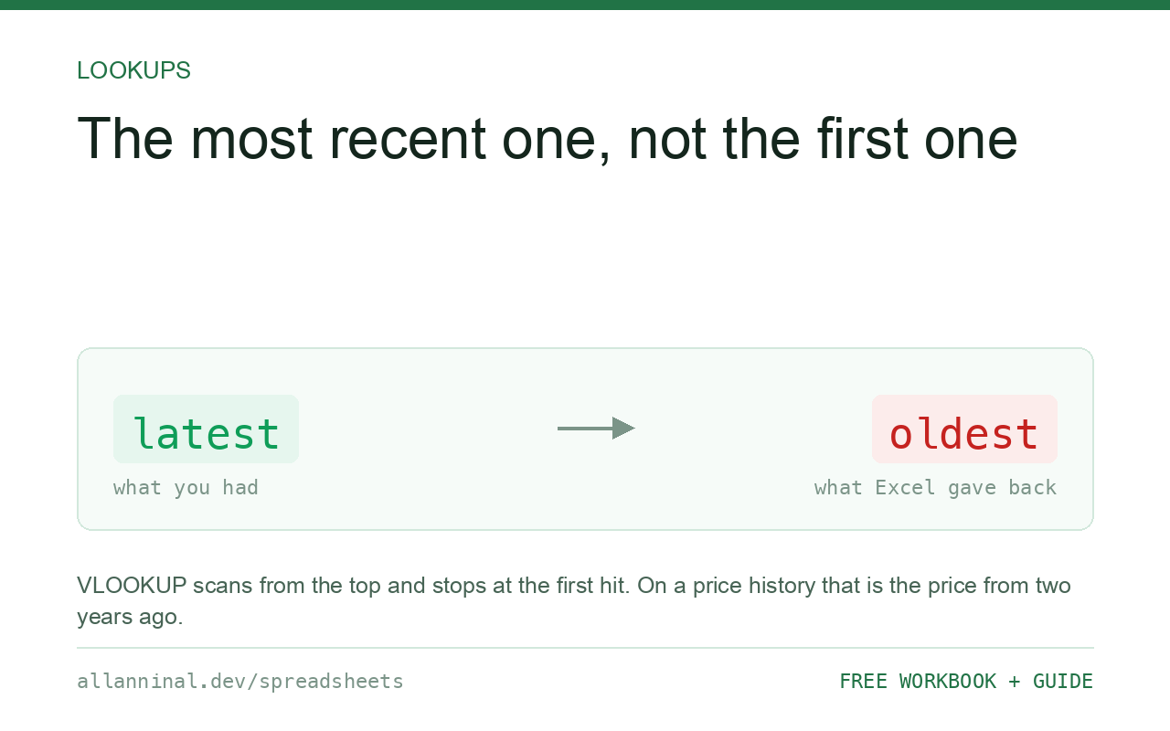
The price list has three rows for the same product because the price changed twice. VLOOKUP hands you the oldest one, because the first match is the only match it knows how to find.
On Excel 365 or 2021, add -1 as XLOOKUP's fifth
argument to search from the bottom up. On any version,
=LOOKUP(2,1/(A:A=key),B:B) returns the last match — an old trick that works
everywhere and reads like nonsense until you know why. Both beat sorting your data backwards, which
solves it once and breaks the next time someone sorts it.
Why first-match is the default, and when that hurts
Most lookups are against a reference table where each key appears once, so first and last are the same thing and the question never arises.
It arises the moment your table is a log rather than a reference: a price history, a status trail, a series of meter readings. There the newest row is the one that matters, and it is at the bottom.
VLOOKUP and MATCH both scan from the top and stop at the first hit. There
is no argument to change that. The fix is either a function that can search backwards, or a
calculation that finds the largest matching position rather than the first.
| What you see | What actually happened | What fixes it |
|---|---|---|
| Getting an old price | First match, and the table is a history | Search from the bottom |
| Status is out of date | Same cause | XLOOKUP with -1 |
| Right until a row was added | The new row is below the one being found | Search from the bottom |
#N/A from the LOOKUP trick | No match at all, or the key type differs | Wrap in IFERROR; check types |
| Correct only while sorted | The workaround was sorting | Use a formula that does not depend on order |
How to find the last matching value
Excel 365 or 2021: XLOOKUP with search mode -1
The fifth argument is the one nobody reads about:
=XLOOKUP(G1,A2:A500,B2:B500,"not found",0,-1)Arguments in order: what to find, where to look, what to return, what if missing,
match mode (0 = exact), search mode (-1 = last to first). The two zeros before it must be
there as placeholders.
Any version: the LOOKUP trick
This appears in workbooks everywhere and almost nobody can explain it:
=IFERROR(LOOKUP(2,1/($A$2:$A$500=G1),$B$2:$B$500),"not found")$A$2:$A$500=G1 gives TRUE and FALSE per row. Dividing 1 by those gives
1 for TRUE and a divide-by-zero error for FALSE. LOOKUP then searches for 2 in a list
whose largest value is 1, never finds it, and by design settles on the last value that was
not an error. That last 1 is the last match.
Add conditions with a second test
The last price for a product from a particular supplier:
=LOOKUP(2,1/(($A$2:$A$500=G1)*($C$2:$C$500=G2)),$B$2:$B$500)Multiplying the two TRUE/FALSE lists gives 1 only where both hold. The rest of the trick is unchanged.
Or find the position, then fetch it
More readable, if longer:
=INDEX($B$2:$B$500,MAX(IF($A$2:$A$500=G1,ROW($A$2:$A$500)-1)))On Excel 2019 and earlier this needs Ctrl+Shift+Enter. The
-1 converts a sheet row number into a position within the range, and getting it wrong by
one is the usual bug here.
Everything on this page, as a workbook you can use on your own data
The Excel Data Cleanup Kit — a seven-tab workbook that finds all nine of these faults in a pasted column and hands back a cleaned version, a five-page PDF guide, and a short read-me. Free, no email required.
- Excel-Data-Cleanup-Workbook-Free.xlsx — paste a column, read the diagnosis, take the cleaned output
- Excel-Data-Survival-Guide.pdf — the eight failures, the import routine that prevents them, every formula explained
Plain .xlsx: no macros, no add-ins. Opens in Excel, Google Sheets,
Apple Numbers and LibreOffice Calc.
Getting the whole row
Wrap the position in INDEX over the full width:
=INDEX($A$2:$F$500,MATCH(2,1/($A$2:$A$500=G1)),0)The 0 as the column argument means “all columns”, so on a modern Excel
the whole row spills.
Sort by date, not by row order
“Last” here means last in the sheet, which is only the most recent if rows were added in date order. If they were not, sort by date first, or find the largest date that matches and look that up instead. This is a real source of quietly wrong answers in workbooks that several people append to.
A dedicated date column beats row position
If “most recent” is the question you keep asking, do not rely on position at all:
=MAXIFS($D$2:$D$500,$A$2:$A$500,G1)That gives the latest date for the key; use it as a second criterion in a
XLOOKUP or SUMIFS to fetch the value. Slower, and it cannot be broken by
somebody sorting the sheet.
Google Sheets
Sheets has no XLOOKUP search mode, but the LOOKUP trick works exactly as
written. QUERY is often clearer there:
=QUERY(A:B,"select B where A='"&G1&"' order by A desc limit 1").
Questions people ask
How do I make VLOOKUP return the last match?
You cannot — VLOOKUP always scans from the top. Use XLOOKUP with search mode -1, or the LOOKUP(2,1/(range=key),result) trick, which works in every version.
How does the LOOKUP(2,1/...) trick work?
Dividing 1 by a TRUE/FALSE list gives 1 for matches and errors for the rest. LOOKUP searches for 2, never finds it, and settles on the last non-error value — which is the last match.
What is XLOOKUP's fifth argument?
Search mode. 1 searches first to last, -1 searches last to first. The match mode argument before it must be supplied as a placeholder.
Does 'last' mean most recent?
Only if rows were added in date order. If they were not, sort by date first, or find the largest matching date with MAXIFS and look that up instead.
Can I get the last match on two conditions?
Yes. Multiply the conditions inside the trick: LOOKUP(2,1/((A=x)*(C=y)),B).
What is the equivalent in Google Sheets?
The LOOKUP trick works unchanged. QUERY is often clearer: select the column, order by descending, limit 1.
Related guides
Take the workbook with you
The Excel Data Cleanup Kit — a seven-tab workbook that finds all nine of these faults in a pasted column and hands back a cleaned version, a five-page PDF guide, and a short read-me. Free, no email required.
- Excel-Data-Cleanup-Workbook-Free.xlsx — paste a column, read the diagnosis, take the cleaned output
- Excel-Data-Survival-Guide.pdf — the eight failures, the import routine that prevents them, every formula explained
Plain .xlsx: no macros, no add-ins. Opens in Excel, Google Sheets,
Apple Numbers and LibreOffice Calc.