Simulator Risk analysis
one number is the least useful answer to a question about risk
A single-figure estimate is a guess wearing a suit. A simulation runs the whole thing a thousand times with every uncertain input varying the way it really varies, and gives you the shape of what could happen — including the tail, which is the part that actually hurts.
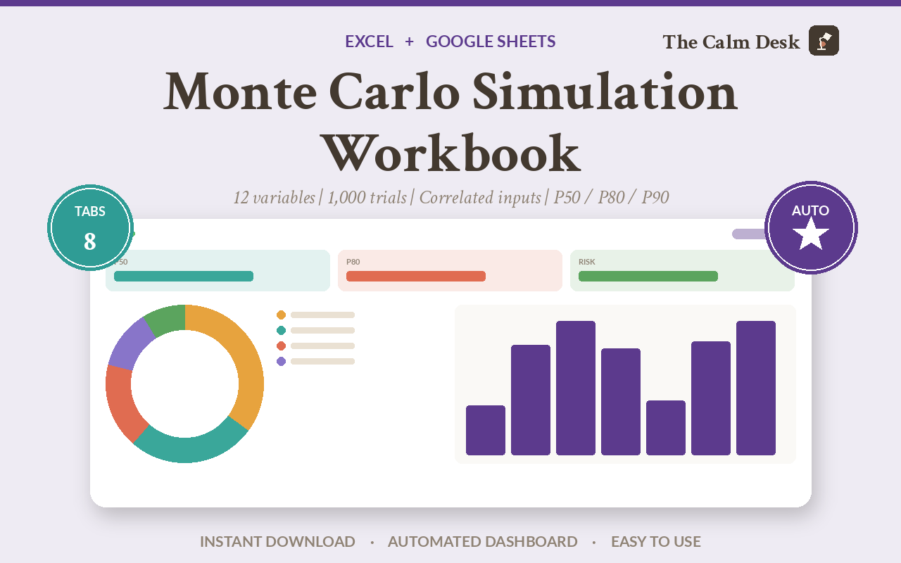
Monte Carlo simulation means running a calculation many times, each time drawing every uncertain input at random from a range you specify, and collecting all the answers. Instead of one number you get a distribution — and from that you can say things like “there is an 80% chance this comes in under budget”.
This workbook does it in ordinary spreadsheet formulas: 12 variables, 1,000 trials, five distributions, and correlation between inputs. No add-in, which is why it also works in Google Sheets and Numbers.
Why the single number is always optimistic
You are estimating a project. Twelve cost items. For each one you write down your best guess, you add them up, and you get a total.
The trouble is that each of those guesses is a range, not a number, and the ranges are not symmetric. Things can go a bit better than expected. They can go enormously worse. Adding up twelve best guesses gives you a total that is roughly the middle, which sounds fine until you notice you have no idea how far the far end is.
And there is a second problem that is easy to miss. Those twelve items are not independent. If steel gets expensive, several of them get expensive together. If the schedule slips, several costs rise at once.
Adding up independent best guesses lets the highs and lows cancel each other out, which makes the total look far more predictable than it is. Correlated inputs do not cancel — they pile up.
How much correlation actually matters
This is the workbook's central claim, so it is asserted by the checker rather than assumed. If you sum inputs that move together, the spread of the total is wider than the independent sum would predict.
| What it assumes | Spread of the total | |
|---|---|---|
| Independent sum | Every input varies on its own | sqrt(sum of the individual variances) |
| This simulation, correlated | Inputs move together, as they really do | 1.59 to 1.64 times wider |
| Understated by | if you ignore correlation | about 60% |
Roughly 60% more spread than an independent model predicts. That gap sits entirely in the tail — which is the region you built the model to understand. An estimate that ignores correlation is not slightly optimistic; it is confidently wrong about exactly the scenario you are trying to protect against.
How it works without an add-in
The whole thing rests on inverse-transform sampling. Every
distribution has an inverse cumulative function; feed it a uniform random number between 0 and 1
and out comes a draw from that distribution. One formula per draw, and
RAND() supplies the uniform number. That is why no add-in is needed.
Correlation uses a single-factor Gaussian copula, which is a fancy name for a simple trick:
Z_i = rho x Z + sqrt(1 - rho^2) x NORMSINV(RAND())
U_i = NORMSDIST(Z_i)
Every variable shares a common factor Z, and takes its own independent part alongside it. Z_i is standard normal by construction, so U_i stays uniform — which means every marginal distribution is preserved exactly and only the joint behaviour changes. Set rho to zero and you get independent sampling back.
The percentiles come from PERCENTILE() over the real trials, never from a normal
approximation. The sum of skewed, correlated inputs is itself skewed, and fitting a normal curve to
it would understate precisely the tail you care about.
How to run a Monte Carlo simulation in a spreadsheet
Describe each input as a range, not a number
Five distributions are available. Triangular when you know the minimum, most likely and maximum — the usual choice for cost and duration estimates. Uniform when anything in a range is equally likely. Normal for measurement-like variation. Lognormal when something cannot go below zero and has a long upper tail. Fixed for things that genuinely do not vary.
Set the correlation
Zero means independent. Higher values tie the variable more tightly to the common factor. This is the step most spreadsheet simulations skip, and it is worth about 60% of the spread of your total.
Run the trials
Every draw is a real cell you can inspect. Nothing is hidden inside an add-in, so if you want to know where a number came from you can follow it.
RAND() is volatile, so pressing F9 reruns the entire simulation. That is a
feature: run it several times and see whether your conclusion is stable.
Read the percentiles, not the mean
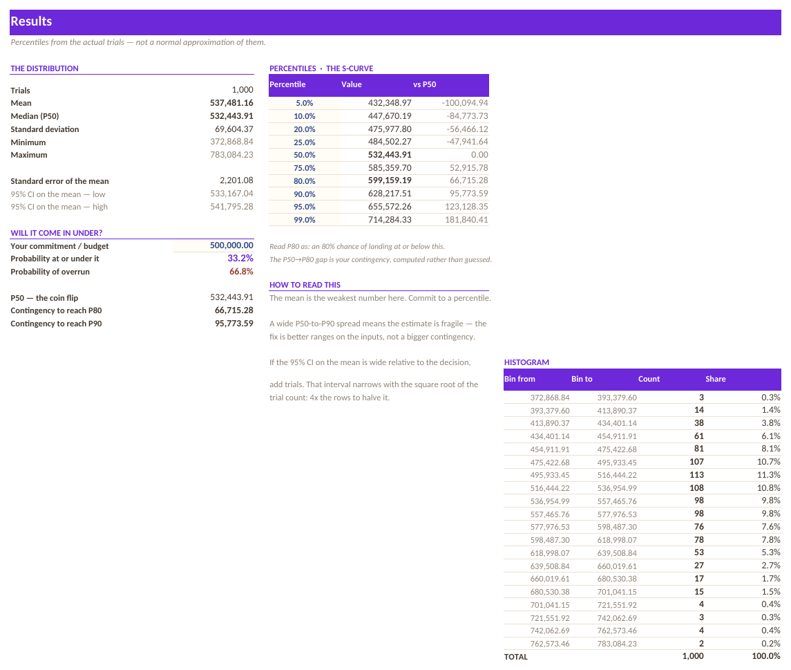
The mean is the least interesting output. What you want is P80: the figure you have an 80% chance of coming in under. That is what you budget to.
The standard error of the mean is shown too, so you can judge whether 1,000 trials was enough rather than assuming it.
Find out which input is driving the spread
Usually two or three inputs dominate. Those are where more research actually pays; tightening your estimate of a variable that contributes 2% of the variance is wasted effort.
To freeze a run for comparison, paste values into the Compare tab — otherwise the next recalculation replaces it.
What is inside the file
Eight tabs. Every random draw is a visible cell, which is unusual: most simulation tools are a black box with a button.
| Tab | What it does |
|---|---|
| Start Here | What to fill in, how to freeze a run, and how to import into Google Sheets. |
| Variables | Your 12 inputs, each with a distribution, its parameters and a correlation. |
| Trials | 1,000 rows of actual draws. Every random number is a cell you can inspect. |
| Results | Mean, standard deviation, percentiles, the S-curve, and the probability of coming in under a threshold you set. |
| Sensitivity | Which inputs contribute most of the variation in the total. |
| Compare | Paste a frozen run here to compare scenarios side by side. |
| Presets | Ready-made setups for common estimating situations. |
| How It Works | The sampling method, the copula, and why percentiles come from the real trials. |
Opening it in Excel, Google Sheets or Numbers
It is one .xlsx file. There are no macros, no add-ins and nothing to install, which is what makes it portable — a macro-driven template would be Excel-only.
| App | How to open it |
|---|---|
| Microsoft Excel | Double-click the file. Excel 2016 and later, and Microsoft 365, on Windows or Mac. Nothing to enable and nothing to install. |
| Google Sheets | Go to Google Drive, click New → File upload and pick the .xlsx. Then double-click it in Drive and choose Open with → Google Sheets. To keep a native copy, use File → Save as Google Sheets. Formatting and formulas both carry over. |
| Apple Numbers (Mac, iPad, iPhone) | Numbers opens .xlsx directly — double-click it, or in Numbers use File → Open and select the file. Numbers converts it on open and will list anything it changed. To send a copy back to someone on Excel, use File → Export To → Excel. |
| LibreOffice Calc | Free, and opens the file as-is on Windows, Mac and Linux. This is what I use to recalculate every workbook when I check the maths, so it is the app these files are tested hardest in. |
This one leans on CORREL, MEDIAN, NORMINV, NORMSDIST, NORMSINV, PERCENTILE, RAND, RANK and STDEV — the functions people most often worry about losing in another app. All of them exist in Excel, Google Sheets, Apple Numbers and LibreOffice Calc, so the file works the same in all four.
Get the workbook
$69 one-off · no subscription
- One .xlsx file, eight tabs, works in Excel, Google Sheets, Numbers and LibreOffice
- 12 variables, 1,000 trials, five distributions
- Correlated inputs via a single-factor Gaussian copula
- Every draw visible as a real cell — no black box
- Sensitivity ranking, S-curve and a Compare tab for frozen runs
- Free lifetime updates
Instant download from Gumroad. RAND() is volatile, so F9 reruns the simulation. Start Here explains how to freeze a run.
The arithmetic, written out
draw            = INVERSE_CDF(distribution, U)      # inverse-transform sampling
U               = RAND(), clamped to [1e-6, 1 - 1e-6]

Z_i             = rho x Z + SQRT(1 - rho^2) x NORMSINV(RAND())
U_i             = NORMSDIST(Z_i)                    # single-factor Gaussian copula

P80             = PERCENTILE(all trial totals, 0.8)
standard error  = STDEV(totals) / SQRT(trials)
U is clamped away from 0 and 1 so the normal inverses stay finite at the extremes — without it a single draw at exactly 0 produces an infinity that poisons the whole run.
And the copula construction is what keeps this honest: because Z_i is standard normal by construction, U_i is uniform, so each variable's own distribution is exactly preserved. The correlation changes how variables move together and nothing else.
How I know the numbers are right
A stochastic model cannot be checked by matching values, so this one is checked by asserting the properties that must hold for a correct sampler and would fail for a broken one. The workbook is recalculated in LibreOffice with real draws.
Last three independent runs: 0 statistical failures, 0 formula errors.
- Every marginal matches theory — mean within five standard errors, standard deviation within 18%, for all 12 variables across triangular, uniform, normal and lognormal. A mis-transcribed inverse CDF fails here immediately
- Hard bounds hold: triangular draws never escape [min, max], lognormal never goes negative
- The shared factor Z is standard normal (mean ~0, sd ~1)
- Correlation actually bites — the observed spread of the total exceeds the independent-sum prediction, by a ratio of 1.59 to 1.64
- Percentiles are monotonic, and the sheet's P50 matches the empirical median
- The histogram accounts for every single trial
- The top sensitivity driver is genuinely among the highest-variance inputs
That histogram assertion caught a real bug. The bins were defined as > lo and
<= hi, which silently drops any trial sitting exactly on a boundary —
including the minimum. Three trials in a thousand were vanishing. The bins now tile
[lo, hi) with the last one closed.
Compared with the alternatives
| Cost | Add-in needed | Correlation | Works in Sheets | |
|---|---|---|---|---|
| This workbook | $69 | No | Yes, copula | Yes |
| @RISK / Crystal Ball | ~$500+ | Yes | Yes | No |
| A three-point estimate | $0 | No | No | Yes |
| A free simulation template | $0 | Sometimes | Almost never | Varies |
Questions people ask before buying
What is Monte Carlo simulation?
Running a calculation many times, drawing each uncertain input at random from a range you specify, and collecting the results. Instead of one estimate you get a distribution, so you can answer questions like 'what figure am I 80 percent likely to come in under'.
Does it need an add-in like @RISK or Crystal Ball?
No. It uses inverse-transform sampling on RAND(), which is ordinary spreadsheet arithmetic. That is why it also works in Google Sheets, Numbers and LibreOffice.
Why does correlation matter so much?
Because correlated inputs do not cancel each other out. If several costs rise together, the total is far more variable than an independent model predicts. Here the observed spread runs 1.59 to 1.64 times the independent-sum prediction — about 60 percent more.
Which distribution should I use?
Triangular when you know minimum, most likely and maximum — the usual choice for cost and duration. Uniform when anything in the range is equally likely. Normal for measurement-like variation. Lognormal when a value cannot go below zero but has a long upper tail.
Why does the answer change every time I edit a cell?
RAND() is volatile, so any recalculation reruns the whole simulation. That is deliberate — press F9 a few times to see whether your conclusion is stable. To freeze a run, paste values into the Compare tab.
Is 1,000 trials enough?
Usually, for planning decisions. The workbook shows the standard error of the mean so you can judge it rather than guess.
Why not just fit a normal curve to the total?
Because the sum of skewed correlated inputs is itself skewed. A normal fit understates exactly the upper tail you built the model to understand. Percentiles here come from the real trials.
Will it work in Google Sheets?
Yes. It uses RAND, NORMSINV, NORMSDIST and PERCENTILE, all of which Sheets and Numbers support.
Related spreadsheets
Ready to stop doing this by hand?
$69 one-off · no subscription
- One .xlsx file, eight tabs, works in Excel, Google Sheets, Numbers and LibreOffice
- 12 variables, 1,000 trials, five distributions
- Correlated inputs via a single-factor Gaussian copula
- Every draw visible as a real cell — no black box
- Sensitivity ranking, S-curve and a Compare tab for frozen runs
- Free lifetime updates
Instant download from Gumroad. RAND() is volatile, so F9 reruns the simulation. Start Here explains how to freeze a run.